Simple Yet Accurate: Calculating a LTV prediction for games, without being a Data Scientist

By Chen Karni, Data Science Director at Plarium

This article is also available in Ukrainian and Russian

One of the most repeated and desired predictions requested by company managers, across a majority of industries, is the calculation of a customer’s LifeTime Value, or in short- LTV.
LTV is usually an assessment of the total revenues expected to be received from a single customer, in the time-span of the customer’s relationship with a product or service, from beginning to end. 
LTV calculation of a customer is often used to assess and measure the profitability of the product over time, and determine which marketing sources or sales techniques eventually bring the highest quality.

There are many ways of calculating this prediction for a product, and specifically for a gaming product. From looking at different player segments, meaning the player’s basic attributes permutation (can be geography, platform, acquisition source, etc), to calculating this value per a single player. Of course, this also determines the level of difficulty and accuracy of the prediction. 
Looking at segments, we can keep this as a mathematical calculation, and produce a number that symbolizes the average revenue amount coming from an average player in that segment. For games with in-game monetization mechanisms, this means the average payments value multiplied by the number of payments that a player is expected to pay during his time in the game until he churns (for further reference, read about the Buy Till You Die model, developed already in 1987).

When looking at the single-player level, this calculation will usually require some kind of machine learning prediction. Meaning, one needs to take into consideration various player factors, including the basic attributes of a segment mentioned above, but focusing on the player behavior in the game, detecting relevant trends that can provide an indication of his future revenues.

Without a doubt, a machine learning prediction is by far more accurate than any high-level calculation. It allows us to differentiate between types of players, and identify trends in their gameplay that can be then used to assess many different aspects. We can determine how long they are going to play the game, to what extent they understand the game, how much time and effort they plan to invest in building up their game assets, and how new game versions or new features or packages in the game, can affect all of the above. However, these models take a long time to develop, they require many resources (a very large amount of data and strong machines to process it), and of course, a data scientist who knows how to bind all of this data into a prediction.

So depending on your task and resources at hand, each game developer should choose how important the LTV calculation is for their specific needs, and how much time and effort they would like to invest in this. The good news is- for many use cases, a simple and high-level calculation can be more than enough to answer most needs. In fact, when properly done, it can be very accurate, with up to 10% margin of error. 

In this post, we would like to focus on a high-level LTV calculation per segment, which can be done in various relatively simple ways, among those, Logarithmic Regression.

What do you need for an LTV Calculation per segment?

Life-Time Span: We need to decide what the relevant time frame is for a player, and for that, we need to understand the player’s activity in the game and the reasonable time in which all deposits will be done until he churns. We will define that as the player’s “life-span”. Depending on the game, this can be a week, a month, and even a few years.

The longer this period is, the harder it is to predict the future, as more and more external and internal variables may change during this long period of time. External variables can be life-changing events (that cause the player to lose interest in the game), world-wide events (such as war, climate disasters, epidemics), professional and economical changes (from changing a job to the economic crisis). Internal and more “controllable” variables can be related to the game itself- added sections, changes in the mechanism, changes to live-ops, new features, and new purchasable packages.

Therefore, we should focus on the time span that will give us the best indication of our revenues, and focus on the majority of the revenues. When do roughly 85% of our revenues happen? That should be the focus time frame.

Data: We need at least a few months of historical data. The granularity of it depends on the relevant time frame: do I want this calculation to be based on daily, weekly, or monthly data? The less relevant data I have, the deeper I would prefer my granularity to be.

If I have data from 5-6 months or more, weekly or monthly granularity would be enough, (depending on the volatility of player deposits). If I have less, daily or weekly granularity would be better.

How do I define relevant data? Data which is relevant to my current product version or offering. If something substantial was changed in my product’s features, in-game packages (subscription, content, or price changes) or appearance, the data might be less indicative and will bring lower accuracy for our calculation.

Understanding what Regression is: Regression is defined as the mathematical relationship found between a group of parameters/variables, allowing us to use available data in order to assess unavailable data. 

In our case, we take existing revenues per player segment and try to assess the amount of future revenues. This can be done using various methods- moving average or linear regression are very popular. In the gaming industry, we can better rely on logarithmic regression when predicting the longer 5-6 months’ time frame.

This means that the relationship between the revenues is assumed to be based on a logarithmic equation, which looks approximately like this:

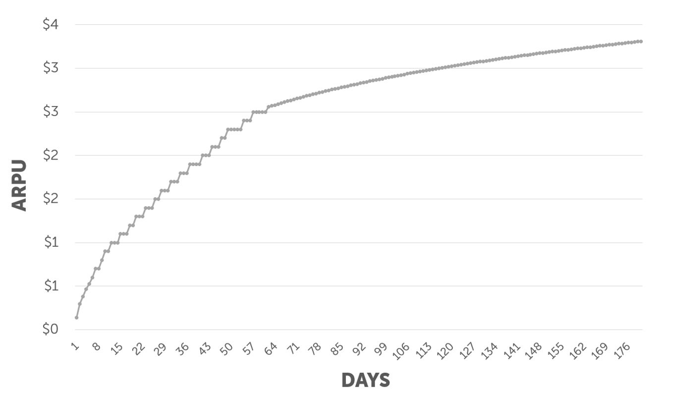
This graph is displaying LTV 180 days prediction, based on the first 60 days.

While the first 60 days of ARPU (Average Revenue Per User) are based on real data, the rest 120 days are based on a natural logarithmic equation of ln(x), which is conjured based on the real data.

How is it done? 

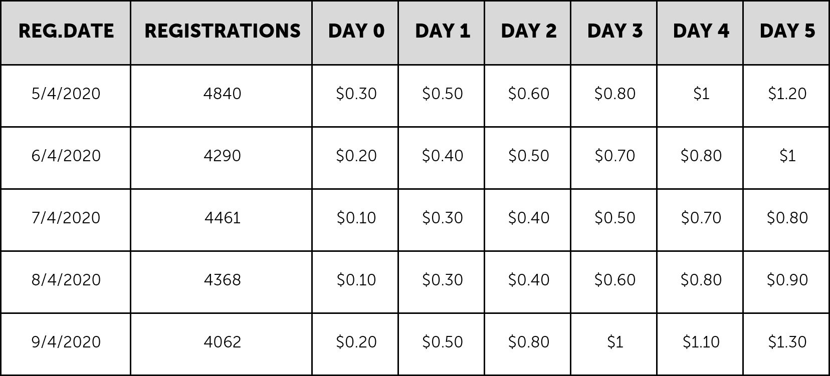
Step One: We need to take the data on which we would like to conduct the calculation. It can either be ARPU or ROAS (Return Over Advertising Spend). We then choose the granularity of our calculation (daily/weekly/monthly) and extract it by cohort. If you take 3 months of daily data, you should get 90 ARPU columns (D0 ARPU, D1 ARPU… D90 ARPU), and 90 rows (for each day).

For example, this is a snapshot of daily ARPU data:

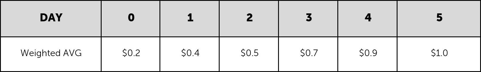
Step Two: We need to run a weighted average calculation, calculating each day’s average ARPU value. This will give us the weighted average value for the first days. Over time the growth rate of each day’s value will usually get lower and lower as we progress on the cohort days.

Step Three: We should remove the top 3-5 and bottom 3-5 dates with the highest and lowest values, to remove the top 5% and bottom 5% outliers which may distort our average trend.

Step Four: Calculate the logarithmic equation describing the given days of our data. This can be done using Excel, R, or Python (using matplotlib.pyplot and scipy.optimize curve_fit could work great), or any statistical analysis software (such as SPSS or MATLAB), depending on your favorite tool of work.

Eventually, either way, you choose, the regression provides a formula in the following structure:

x represents the number of days, for example, for ARPU day 3. x = 3
y represents the final ARPU received per a given day x, for example, ARPU day 61 equation output.

On the data provided above, this is the logarithmic formula I received:

Using my original example, in order to predict the 60+ days of the ARPU, we can use the formula received above.

We will use the calculated average for the first 60 days as real data, and then we will continue the following days, feeding x as the day number.

Sometimes the formula will require some manual adjustments. One parameter to adjust can be the y axis intercept (the b parameter in the equation described above), to heighten or lower the equation line to best fit the real data curve. Another can be the point in time where revenue growth starts to decay. In case this time is later than the chosen real data time frame (in the example above it is 60 days), one might consider making a combination with another formula type that might predict the revenue better, such as linear regression.

Now, all that is left is to play with the data, cut it into different segments and understand the differences, and compare it with CPI (Cost Per Install) rates in order to understand the game’s profitability status.

We recommend to repeat this calculation periodically and see how the profitability of the game changes, which can also help us identify when player acquisition might not be worthwhile.

Go ahead and try it out!